IP and EA for molecule (N2)

Example on computing ionization potential and electron affinity from self-consistent GW for Nitrogen molecule

Here we provide a simple example on how to run Green/Weakcoupling for computing ionization potential (IP) for nitrogen molecule (Geometry obtained for GW100 dataset). Prerequisites: you must have the mbpt compiled and the green-mbtools python package installed. Change to a new directory where you will keep your simulations, create a directory for the $N_2$ simulation. Then create a file with the atom positions in the atom.dat:

N 0.0000 0.0000 0.0000
N 0.0000 0.0000 1.0977

The remaining parameters will be specified on the command line.

We then obtain input parameters and the initial mean-field solution by running pySCF via the init_data_mol_df.py script:

python <source root>/green-mbpt/python/init_data_mol_df.py        \
  --atom atom.dat --basis ccpvdz --xc PBE0

We use the ccpvdz basis-set and hybrid PBE0 exchange correlation potential as reference. Not specifying the xc would run Hartree-Fock.

The primary goal of this example is to run a molecular example using fully self-consistent GW and perform analytical continuation to obtain photoelectron spectra and IP.

After that we will run the GW approximation

<install dir>/bin/mbpt.exe --scf_type=GW --BETA 1000              \
  --grid_file ir/1e5.h5 --itermax 40 --results_file sim.h5        \
  --mixing_type CDIIS --diis_start 2 --diis_size 5 --mixing_weight 0.3 \
  --jobs SC

Here we run the self-consistent GW approximation at inverse temperature $\beta=1000$ , we use an IR nonuniform grid for $\Lambda = 10^5$ .

<install dir>/bin/mbpt.exe --scf_type=GW --BETA 1000                    \
  --grid_file ir/1e5.h5 --itermax 40 --results_file sim.h5              \
  --mixing_type CDIIS --diis_start 2 --diis_size 5 --mixing_weight 0.3 \
  --jobs SC,WINTER                \
  --kernel GPU --cuda_low_gpu_memory true --cuda_low_cpu_memory true

Here we run the self-consistent GW approximation at inverse temperature $\beta=1000$ , we use an IR nonuniform grid for $\Lambda = 10^5$ .

We set value for --kernel to GPU to run CUDA implementation. We set both CPU (--cuda_low_cpu_memory true) and GPU (--cuda_low_gpu_memory true) memory to low to avoid excessive memory allocation.

We then store results into sim.h5 file.

Now we will use the green-mbtools package to perform Nevanlinna analytical continuation from the imaginary axis to real axis.

python <source root>/green-mbtools/examples/nvnl_analysis_mol.py --input input.h5 --sim sim.h5 --iter -1  --beta=1000 \
   --grid_file ir/1e5.h5  --out ac_out.h5 \
   --e_min -5.0 --e_max 5.0 --n_omega 4000 --eta 0.01

This will run Nevanlinna analytical continuation for the data obtained at the last iteration. The output will be stored in the group ac_out.h5.

A plot for the specrta can then be obtained with the plot_dos_mol.py script:

python <source root>/green-mbtools/examples/plot_dos_mol.py --ac_out nvnl_out.h5

This will read the analytically continued data and plot it to an <output_dir>/spectra.pdf file. In addition, it will also print the ionization potential (IP) and elecrton affinites (EA). The resultant spectra looks like:

alt text

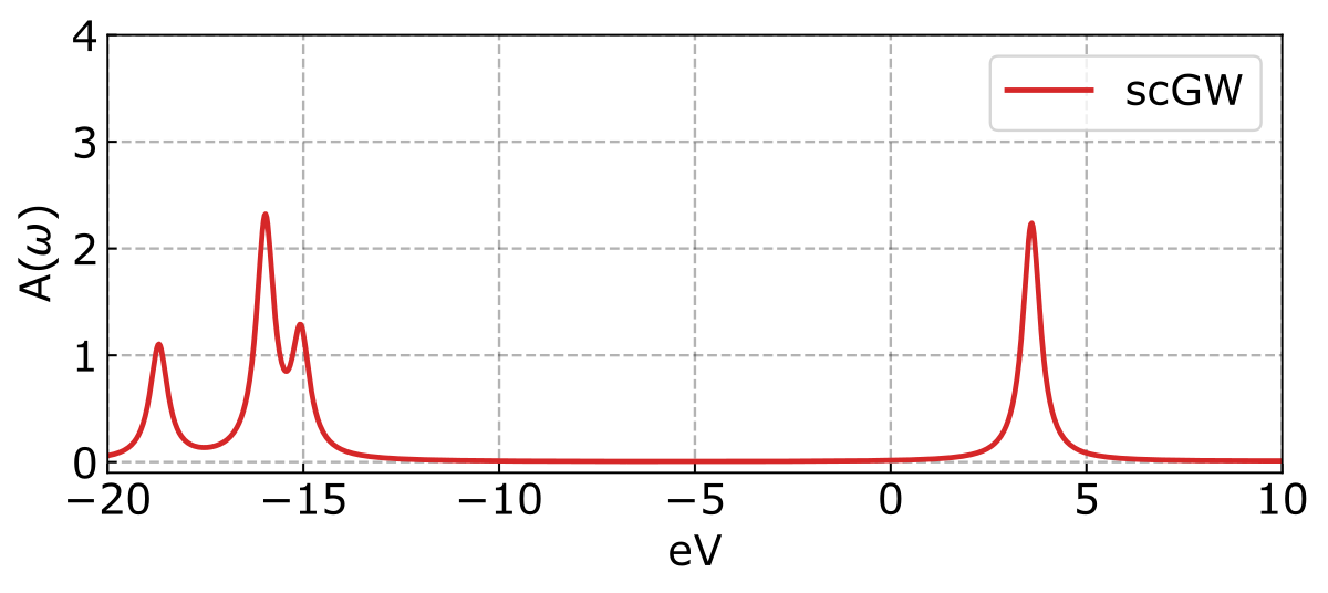
And the ionization potentials (IP) and electron affinities (EA) are displayed as follows.

Lowest 4 Ionization Potentials:
GW IP 1:  -15.964 eV
GW IP 2:  -15.964 eV
GW IP 3:  -15.066 eV
GW IP 4:  -18.685 eV

Lowest 4 Electron Affinities:
GW EA 1:    3.604 eV
GW EA 2:    3.604 eV
GW EA 3:   15.143 eV
GW EA 4:   21.321 eV

It is important to highlight that the quasiparticle energies are ordering according to the mean-field reference. As a result, the quasiparticle energies may not be arranged in increasing order because of corrections from dynamic self-energy.

Post-processing SEET embedding