GW band structure (Si)

Example to compute GW band structure

Here we provide a simple example on how to run Green/Weakcoupling on the example of a periodic silicon on 6x6x6 lattice. Prerequisites: you must have both the mbpt and the ac executables compiled, and the green-mbtools python package installed. Change to a new directory where you will keep your simulations, create a directory for the Si simulation, and create the file a.dat containing the following unit cell information:

0.0,  2.7155, 2.7155
2.7155, 0.0,  2.7155
2.7155, 2.7155, 0.0

Then create a file with the atom positions in the atom.dat:

Si 0.0  0.0  0.0
Si 1.35775 1.35775 1.35775

The remaining parameters will be specified on the command line.

We then obtain input parameters and the initial mean-field solution by running pySCF via the init_data_df.py script:

python <source root>/green-mbpt/python/init_data_df.py        \
  --a a.dat --atom atom.dat --nk 6                            \
  --basis gth-dzvp-molopt-sr --pseudo gth-pbe --xc PBE

Here we use the gth-dzvp-molopt-sr basis with the gth-pbe psudopotential and run DFT mean-field approximation with a PBE exchange correlation potential.

The primary goal of this example is to generate the band structure of Silicon. For that, we require the overlap matrix and one-electron Hamiltonian along the high-symmetry path in addition to the density functional solution. We set the high-symmetry path to WGXWLG to reproduce the results from [Phys. Rev. B 106, 235104]. To calculate these quantities, we run the script init_data_df.py again, but this time with an additional --job sym_path flag:

python <source root>/green-mbpt/python/init_data_df.py        \
  --a a.dat --atom atom.dat --nk 6                            \
  --basis gth-dzvp-molopt-sr --pseudo gth-pbe --xc PBE        \
  --job sym_path --high_symmetry_path WGXWLG  --high_symmetry_path_points 100

Note that it is possible to run both jobs at once using the flag --job init sym_path.

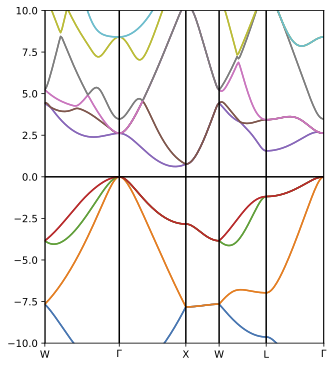
This marks the completion of input data generation and initial mean-field calculation. Before running the GW calculation, it is informative to analyse the mean-field band structure. There are several different ways to obtain the band structure from a converged DFT or HF calculation. Perhaps the fastest approach is to perform k-point interpolation using the green-mbtools python package. Specifically, we can use the [wanner_fock.py for Silicon in the following manner:

python wannier_fock.py --input input.h5 --celltype 'fcc' --bz_type 'fcc' \
  --bandpath 'W G X W L G' --bandpts 100

The resultant band structure (saved as a PDF file) is expected to look like:

alt text

We will now run the GW approximation:

<install dir>/bin/mbpt.exe --scf_type=GW --BETA 100              \
  --grid_file ir/1e4.h5 --itermax 20 --results_file Si.h5        \
  --mixing_type CDIIS --diis_start 2 --diis_size 5 --mixing_weight 0.3 \
  --high_symmetry_output_file Si_hs.h5 --jobs SC,WINTER

Here we run the self-consistent GW approximation at inverse temperature $ \beta=100 $, we use an IR nonuniform grid for $ \Lambda = 10^4 $ and run for no more than 20 iterations.

<install dir>/bin/mbpt.exe --scf_type=GW --BETA 100                    \
  --grid_file ir/1e4.h5 --itermax 20 --results_file Si.h5              \
  --mixing_type CDIIS --diis_start 2 --diis_size 5 --mixing_weight 0.3 \
  --high_symmetry_output_file Si_hs.h5 --jobs SC,WINTER                \
  --kernel GPU --cuda_low_gpu_memory true --cuda_low_cpu_memory true   \
  --Sigma_sp=true --P_sp=true

Here we run the self-consistent GW approximation at inverse temperature $ \beta=100 $, we use an IR nonuniform grid for $ \Lambda = 10^4 $ and run for more than 20 iterations.

We set value for --kernel to GPU to run CUDA implementation. We set both CPU (--cuda_low_cpu_memory true) and GPU (--cuda_low_gpu_memory true) memory to low to avoid excessive memory allocation.

If you are running this on a consumer GPU, floating point operations are often much faster in single precision than in double precision. We therefore additionally force the code to run in single precision:

  --Sigma_sp=true --P_sp=true

such that both the calculation of the self-energy and of the polarization are performed in single precision. Note that on consumer cards such as Nvidia’s Ampere generation, single precision is 64x faster than double precision.

We then store bulk results into Si.h5 file. After the self-consistent simulation is finished band-path interpolation along the high-symmetry path will be evaluated and stored in Si_hs.h5.

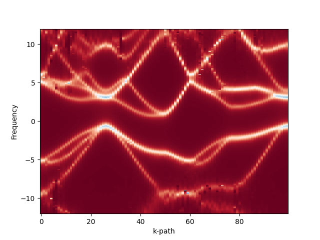
To obtain the spectral function for silicon run

<install dir>/bin/ac.exe  --BETA 100 --grid_file ir/1e4.h5    \
   --input_file Si_hs.h5 --output_file ac.h5 --group G_tau_hs \
   --e_min -5.0 --e_max 5.0 --n_omega 4000 --eta 0.01 \
   --kind Nevanlinna

This will run Nevanlinna analytical continuation for the data obtained at the last iteration for all k-points. The output will be stored in the group G_tau_hs of the output HDF5 file ac.h5.

A plot for the band structure can then be obtained with the plot_bands.py script:

python <source root>/green-mbpt/python/plot_bands.py \
        --input_file ac.h5 --output_dir bands

This will read the analytically continued data and plot it to an <output_dir>/bands.png file. In addition, it will create a plain-text data file for every k-point along the chosen path inside the <output_dir> directory. The expected band structure plot should look as following

alt text

Post-processing