DIIS Tutorial
DIIS tutorial from Pavel Pokhilko.
Simple example: Silicon (Si)
Silicon (Si) is suitable as a convenient pedagogical system for showing how to run DIIS. As per usual, we start from integral preparation with the PySCF library.
Integral preparation
The files below set up the cell vectors and the coordinates, respectively:
a.dat:
0.0,  2.7155, 2.7155
2.7155, 0.0,  2.7155
2.7155, 2.7155, 0.0atoms.dat:
Si 0.0  0.0  0.0
Si 1.35775 1.35775 1.35775
Then a PySCF script, which will prepare the integrals, can be executed:
export OMP_NUM_THREADS=64 # OpenMP multithreading
python3 <source root>/green-mbpt/python/init_data_df.py          \
   --a a.dat --atom atoms.dat --nk 2 --pseudo gth-pbe            \
   --basis gth-dzvp-molopt-sr --auxbasis def2-svp-ri --df_int 1 --spin 0
The command above prepares integrals for Si using a 2x2x2 Monkhorst–Pack k-point grid. Although this grid is quite small, it is fine for our pedagogical purposes. The selected auxiliary basis set works reasonably well for periodic solid calculations containng light elements, such as Si.
DIIS execution
An example of a slurm script is below:
#!/bin/bash

#SBATCH -N 1
#SBATCH -C gpu
#SBATCH -q debug
#SBATCH -J Si
#SBATCH -t 00:30:00
#SBATCH --hint=nomultithread
#SBATCH --gpus-per-node=1

#OpenMP settings:
export OMP_NUM_THREADS=1
export HDF5_USE_FILE_LOCKING=FALSE
export HDF5_DISABLE_VERSION_CHECK=1

export GREEN_INSTALL=<path-to-installed-green-mbpt>
export GREEN_GRID=$GREEN_INSTALL/share/ir
export INTS=<path-to-generated-integrals>

date

srun -n 64 $GREEN_INSTALL/bin/mbpt.exe --scf_type=GW --BETA 300       \
  --grid_file $GREEN_GRID/1e5.h5 --itermax 100 --results_file Si.h5 \
  --input_file $INTS/input.h5 \
  --jobs SC   \
  --diis_start  2 \
  --diis_size  7 \
  --verbose 4 \
  --mixing_type CDIIS --mixing_weight 0.3  \
  --dfintegral_hf_file="$INTS/df_hf_int"  \
  --dfintegral_file="$INTS/df_int" \
  --kernel GPU --cuda_low_gpu_memory true --cuda_low_cpu_memory true >& Si_NEW.txt
Here, --diis_start defines the iteration at which DIIS will start, --diis_size defines the maximum size of the DIIS subspace, --versbose determines how verbose the output will be (large values are useful for troubleshooting), --mixed_type determines which mixing will be used (DIIS for difference residuals and CDIIS for commutator residuals), --mixing_weight is used only for the first few iterations before building the DIIS subspace.
CDIIS often converges faster than DIIS with the difference residuals and simple mixing. However, if very tight convergence criteria are used, CDIIS commutators may become sensitive to numerical noise (see our original paper), and switching to a simple mixing is recommended.
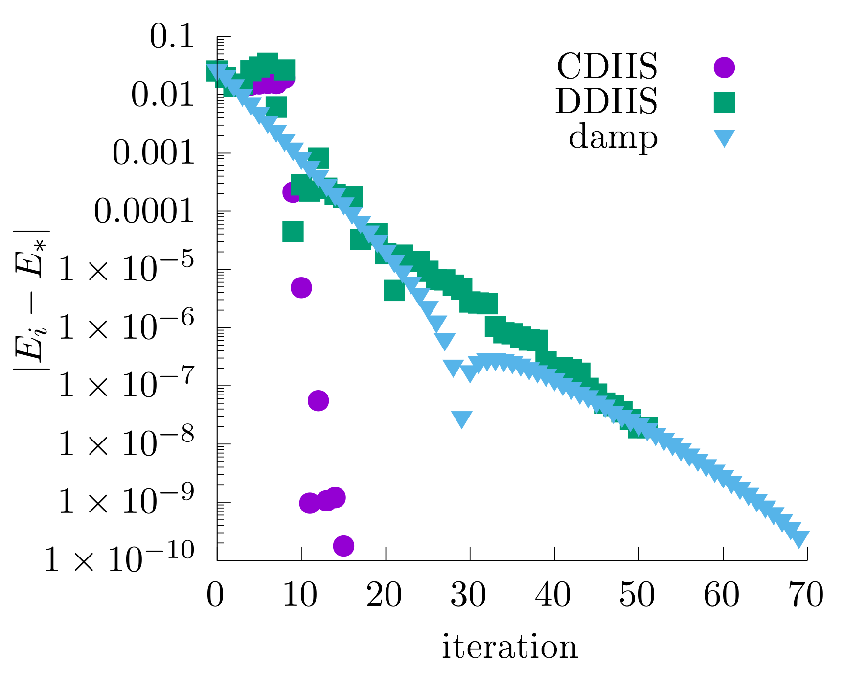
This is a comparison of different algorithms (Sigma mixing, DIIS, CDIIS) with the same settings as above:
Advanced example: BiVO3
BiVO3 is an interesting realistic system that we studied before as a test case of our algorithms:
https://pubs.aip.org/aip/jcp/article/156/9/094101/2840744
It shows an interesting convergence pattern, and can serve as a good example on how to converge iterations. Thanks to Yanbing for sharing geometries and basis sets!
Integral preparation
As per usual, we need to generate integrals first. However, there are only very few basis sets available for Bismuth (Bi). For solids, we commonly use basis sets from the molopt family with gth pseudopotentials. However, MolSSI’s Basis Set Exchange library lack some of these basis sets. We can, for example, download the missing basis sets from CP2K:
https://pierre-24.github.io/cp2k-basis/developers/library_content
Then get the necessary basis sets and save them into the corresponding files, for example:
Bi_basis:
 Bi TZVP-MOLOPT-SR-GTH TZVP-MOLOPT-SR-GTH-q5
 1
 2 0 2 5 3 3 1
      1.66692829 -0.36896598 -0.13784534  0.01904790 -0.08133298  0.12465455  0.08937937 -0.15628186
      1.31794172  0.60312607  0.24301591 -0.07495626  0.24674021 -0.16489926 -0.06073193  0.26733662
      0.22222138 -0.51586411 -0.32950897  0.27952407 -0.92969758  0.19556854 -0.12518709 -0.75590352
      0.07452444 -0.43811758  0.89405382 -0.00047494 -0.09939405 -0.01225247  0.98609977 -0.39542603
      0.06672543 -0.20503722 -0.11846324 -0.95701871  0.24142794  0.95857827  0.01607445 -0.41994669
#V_basis:
V TZVP-MOLOPT-SR-GTH TZVP-MOLOPT-SR-GTH-q13
 1
 2 0 3 6 4 3 3 1
      7.98462375  0.02087541 -0.00975098  0.02120107  0.03099923 -0.17157839 -0.01684344  0.01682335  0.09036199 -0.01161683  0.09137089 -0.00318569
      4.19216995  0.42475532 -0.25067357  0.26611498  0.33725015  0.19107997 -0.00355376 -0.01871944  0.30728774  0.04029333  0.33566567 -0.01236813
      1.67440329 -0.60690412  0.29451036 -0.14319412 -0.33682980  0.66551468 -0.01422047  0.37747378  0.49587427  0.03394291  0.72419759 -0.18175053
      0.66666458 -0.61757168 -0.08479144  0.28100055  0.72222853  0.63922519 -0.06264901  0.02670691  0.67892663 -0.28749821 -0.52617981 -0.77180670
      0.24241988  0.09883238  0.10332899 -0.87706388  0.45031275  0.23669763  0.69335240 -0.66031685  0.43624695  0.41501290 -0.26308693 -0.58022549
      0.06739027  0.24423739  0.91239512  0.24500289  0.21783356 -0.16280323  0.71752282  0.64818862 -0.01627523  0.86150940 -0.09185774 -0.18562438
#O_basis:
#BASIS SET
 O  DZVP-MOLOPT-SR-GTH DZVP-MOLOPT-SR-GTH-q8
 1
 2 0 2 5 2 2 1
     10.389228018317  0.126240722900  0.069215797900 -0.061302037200 -0.026862701100  0.029845227500
      3.849621072005  0.139933704300  0.115634538900 -0.190087511700 -0.006283021000  0.060939733900
      1.388401188741 -0.434348231700 -0.322839719400 -0.377726982800 -0.224839187800  0.732321580100
      0.496955043655 -0.852791790900 -0.095944016600 -0.454266086000  0.380324658600  0.893564918400
      0.162491615040 -0.242351537800  1.102830348700 -0.257388983000  1.054102919900  0.152954188700
#
The saved files above contain basis sets in the CP2K format, while our generating script understands basis sets written in NWChem format. One can either edit the python script using some of PySCF’s libraries to feed the CP2K format (beware of this bug), or convert them in a cleaner way using the MolSSI tools as described here:
https://molssi-bse.github.io/basis_set_exchange/conversion.html
In our case, the user can execute the following commands performing conversion:
  bse convert-basis --in-fmt cp2k --out-fmt nwchem Bi_basis Bi_basis_nwchem
  bse convert-basis --in-fmt cp2k --out-fmt nwchem V_basis V_basis_nwchem
  bse convert-basis --in-fmt cp2k --out-fmt nwchem O_basis O_basis_nwchem
These commands will create Bi_basis_nwchem, V_basis_nwchem, and O_basis_nwchem file with the basis sets in NWChem format.
Then we will need the crystal cell geometry a.dat and the atom positions atoms.dat:
a.dat:
0.392700000000E+01   0.000000000000E+00   0.000000000000E+00
0.000000000000E+00   0.392700000000E+01   0.000000000000E+00
0.000000000000E+00 0.000000000000E+00 0.785400000000E+01atoms.dat:
V     1.963500000000E+00  1.963500000000E+00 -1.9635000
V     1.963500000000E+00  1.963500000000E+00  1.9635000
BI    0.000000000000E+00  0.000000000000E+00  0.0000000
BI    0.000000000000E+00  0.000000000000E+00  3.9270000
O     0.000000000000E+00  1.963500000000E+00 -1.9635000
O     0.000000000000E+00  1.963500000000E+00  1.9635000
O     1.963500000000E+00  0.000000000000E+00 -1.9635000
O     1.963500000000E+00  0.000000000000E+00  1.9635000
O     1.963500000000E+00  1.963500000000E+00  0.0000000
O     1.963500000000E+00  1.963500000000E+00  3.9270000
Then, the actual PySCF script can be executed:
export OMP_NUM_THREADS=64 # OpenMP multithreading
python3 <source root>/green-mbpt/python/init_data_df.py          \
   --a a.dat --atom atoms.dat --nk 2                             \
   --basis 'Bi' 'Bi_basis_nwchem' 'V' 'V_basis_nwchem'           \
   'O' 'O_basis_nwchem' --pseudo gth-pade --xc pbe0  --beta 3.0  --df_int 1
Here, I generate an even-tempered auxiliary basis sets, which is usually very good, but large. In order to reduce the number of auxiliary basis functions, this example uses --beta 3.0. In this pedagogical example, PySCF HF iterations converge quickly, which is sometimes not the case in practice.
Warning! Unfortunately, the default range-separated integrals from PySCF often lead to problematic (or even incorrect) behavior of Green’s function calculations, especially for heavy elements. Please make sure that all the integrals come from pyscf.pbc.df.gdf_builder._CCGDFBuilder. This patch explicitely disables flags from range-separation and gives the desired integrals (tested with PySCF 2.5.0):
https://github.com/Green-Phys/green-mbpt/pull/12
The DFT calculation converges rather quickly. This is not the case for the GW calculations.
GW iterations
The calculaiton can be executed as shown in this script:
export OMP_NUM_THREADS=1
export HDF5_USE_FILE_LOCKING=FALSE
export HDF5_DISABLE_VERSION_CHECK=1

export GREEN_INSTALL=<path-to-installed-green-mbpt>
export GREEN_GRID=$GREEN_INSTALL/share/ir
export INTS=<path-to-generated-integrals>

srun -n 128 $GREEN_INSTALL/bin/mbpt.exe --scf_type=GW --BETA 300       \
  --grid_file $GREEN_GRID/1e5.h5 --itermax 100 --results_file BiVO3.h5 \
  --input_file $INTS/input.h5 \
  --jobs SC   \
  --diis_start  3 \
  --verbose 4 \
  --diis_size  5 \
  --mixing_type CDIIS --mixing_weight 0.5  \
  --dfintegral_hf_file="$INTS/df_hf_int"  \
  --dfintegral_file="$INTS/df_int" \
  --kernel GPU --cuda_low_gpu_memory true --cuda_low_cpu_memory true
In this example, I compare mixing iterations with DIIS and CDIIS. For a fair comparison, I used exactly the same settings for DIIS with the difference residuals and CDIIS as shown in the snippet above. Convergence by total energy is shown in this graph:
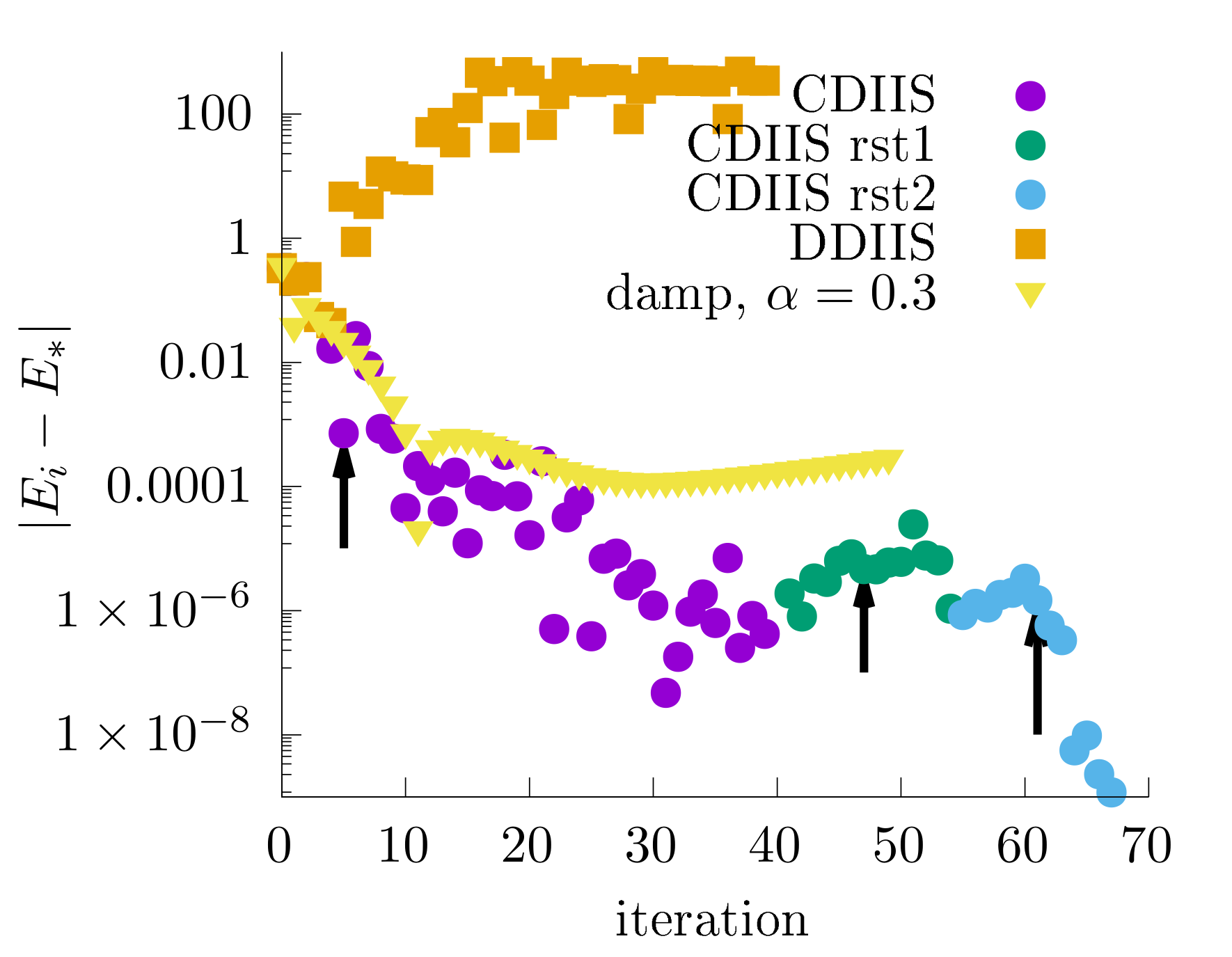
The difference residuals quickly lead to diverging iterations. The mixing iterations (with --mixing_weight 0.3) initially look to be on a convergence path, but after some point, the calculation will start to gradually diverge. CDIIS is much more superior to mixing and DIIS with the difference residuals. In the plot above, I mark the iterations that start CDIIS extrapolations with arrows.
To estimate whether the extrapolation subspace is good, I recommend to look at the printed extrapolation coefficients. They can also help troubleshoot problematic cases. The first iteration with the CDIIS extrapolation has these extrapolation coefficients:
DIIS: Extrapolation coefs:
(0.0587986963467374,0)        <--- the oldest vector
(0.13825987924904,0)
(0.63053206432372,0)
(0.172409360080503,0)         <--- the newest vector
A stable iteration has small coefficients for all vectors. In addition, stable iterations have decaying coefficients for old vectors, makeing it possible to kick out the oldest vectors from the subspace when the maximum subspace size is reached. The magnitude of the first coefficient tells how much it is damped by the CDIIS extrapolation. Often, the coefficients of the newest vectors for smooth stable iterations are about the same from iteration to iteration. However, in the next iteration, I see this picture:
DIIS: Extrapolation coefs:
(0.0588596838465215,0)        <--- the oldest vector
(0.463919504411638,0)
(0.99437078912762,0)
(0.0746981714255306,0)
(-0.591848148811311,0)        <--- the newest vector
The occurrence of the negative coefficient for the newest vector tells that the optimization problem has some curvature, which the quasi-Newton nature of CDIIS attempts to overcome. This curvature is the reason why the mixing iterations will start divering at some point.
Noise troubleshooting
However, CDIIS can be quite noisy as the plot shows. This noise has several origins:
- Bad condition number of the overlap matrix, preventing an accurate solution of the linear system.
- Occurrence of bad vectors in the subspace that are not completely removed from extrapolation by approximate commutator measure of error.
- Important vectors are kicked out from the subspace as iterations go.
- Limitation of the double precision arithmetic at the subtraction operation.
While the precise origin and troubleshooting is problem-dependent, I can provide a general recommendation. When such a noise occurs, I recommend to restart the calculation. One can switch to mixing if it is convergent. For CDIIS, I recommend to restart and rebuild the subspace. Such a restart will kick out the bad vectors, and supply a much better approximation to the Hessian.
Once again, extrapolation coefficients tell a story helping to troubleshoot calculations. At the last few iterations from the first CDIIS run, the coefficients are:
DIIS: Extrapolation coefs:
(1.20971008021554,0)
(-0.408662551765205,0)
(1.74343656638734,0)
(-6.2065904736162,0)
(4.66210637877853,0)
DIIS: Extrapolation coefs:
(2.14087187639123,0)
(-1.86517350134611,0)
(-3.07182955581453,0)
(3.23509473198939,0)
(0.561036448780016,0) DIIS: Extrapolation coefs:
(0.696140249974835,0)
(-5.47256197558599,0)
(4.40368599268861,0)
(0.833342797292691,0)
(0.539392935629858,0) DIIS: Extrapolation coefs:
(-3.45621925669398,0)
(2.87958829836786,0)
(0.499382192840323,0)
(0.397620567653019,0)
(0.679628197832773,0) DIIS: Extrapolation coefs:
(0.0303535900389646,0)
(-0.486327339731549,0)
(0.0906193985714284,0)
(-0.278956640851003,0)
(1.64431099197216,0) We can see in these iterations, that:
- Coefficients of the newest vectors vary substantially.
- Coefficients of the oldest vectors are large.
Therefore, it is reasonable to restart CDIIS, rebuild the subspace (to kick out problematic vectors), and continue with a bigger extrapolation subspace to prevent removal of important vectors. I executed it as follows:
srun -n 128 $GREEN_INSTALL/bin/mbpt.exe --scf_type=GW --BETA 300       \
  --grid_file $GREEN_GRID/1e5.h5 --itermax 100 --results_file BiVO3.h5 \
  --input_file $INTS/input.h5 \
  --jobs SC   \
  --diis_start  5 \
  --restart true \
  --verbose 4 \
  --diis_size  10 \
  --mixing_type CDIIS --mixing_weight 0.1  \
  --dfintegral_hf_file="$INTS/df_hf_int"  \
  --dfintegral_file="$INTS/df_int" \
  --kernel GPU --cuda_low_gpu_memory true --cuda_low_cpu_memory true
This restart is shown in the figure as “CDIIS rst1”. The first few iterations start to diverge despite a substantial applied iteration mixing. When CDIIS starts, it corrects the gradually diverging subspace (and this is also why a bigger subspace is needed here). It substantially de-noises the iterations and leads to a faster convergence of the chemical potential. Unfortunately, the quick queue on the cluster killed my job, so I decided to restart again (“CDIIS rst2”) with even bigger subspace.
srun -n 128 $GREEN_INSTALL/bin/mbpt.exe --scf_type=GW --BETA 300       \
  --grid_file $GREEN_GRID/1e5.h5 --itermax 100 --results_file BiVO3.h5 \
  --input_file $INTS/input.h5 \
  --jobs SC   \
  --diis_start  5 \
  --restart true \
  --verbose 4 \
  --diis_size  20 \
  --mixing_type CDIIS --mixing_weight 0.1  \
  --dfintegral_hf_file="$INTS/df_hf_int"  \
  --dfintegral_file="$INTS/df_int" \
  --kernel GPU --cuda_low_gpu_memory true --cuda_low_cpu_memory true
Once again, slow divergence of mixing is stopped by CDIIS. This subspace has led to very quick convergent iterations without noise.